Time Series Analysis and Anomalies Visualization
MSTICPy has functions to calculate and display time series decomposition results. These can be useful to spot time-based anomalies in something that has a predictable seasonal pattern.
Warning
This document is in the process of being updated The first sections describe some of the new functionality in MSTICPy 2.0 - main the encapsulation of many of the time series functions in pandas accessors. The second part of the document is the original document that is still to be updated.
Some examples are number of logons or network bytes transmitted per hour. Although these vary by day and time of day, they tend to exhibit a regular recurring pattern over time. Time Series decomposition can calculate this seasonal pattern. We can then use this established pattern to look for periods when significant differences occur - these might be indicators of malicious activity on your network.
- Time Series analysis generally involves these steps
Generating TimeSeries Data
Using Time Series Analysis functions to discover anomalies
Visualizing Time Series anomalies
You can read more about time series analysis in detail some Microsoft TechCommunity blog posts.
Looking for unknown anomalies - what is normal? Time Series analysis & its applications in Security
Time Series visualization of Palo Alto logs to detect data exfiltration
Some useful background reading on Forecasting and prediction using time series here Forecasting: Principals and Practice The section dealing with STL (Seasonal and Trend decomposition using Loess) STL decomposition is directly related to the techniques used here.
Preparation
You need to have the SciPy and Statsmodels packages installed to use the Time Series functionality.
An easy way to get these is to install MSTICPy with the “ml” extract
python -m pip install msticpy[ml]
Initializing MSTICPy
import msticpy as mp
mp.init_notebook()
Retrieving data to analyze
Time Series is a series of data points indexed (or listed or graphed) in time order. The data points are often discrete numeric points such as frequency of counts or occurrences against a timestamp column of the dataset.
The basic characteristics of the data that you need is as follows:
Time column - with the time stamp of the sampling interval
A numeric count or sum of whatever value you want to check for anomalies. For example, bytes per hour. The numeric value is calculated for each time period.
The total time span of the data must cover one or more seasonal periods, for example, 7 days.
A simple query for doing this for logon data is shown below.
query = """
SecurityEvent
| where EventID == 4624
| where TimeGenerated >= datetime(2022-05-01 00:00)
| where TimeGenerated <= datetime(2022-06-01 00:00)
| summarize LogonCount=count() by bin(TimeGenerated, 1h)
| project TimeGenerated, LogonCount
"""
ts_df = qry_prov.exec_query(query)
ts_df = ts_df.set_index("TimeGenerated")
Performing the Time Series analysis
MSTICPy has a timeseries module that uses Statsmodel’s STL function to generate the time series analysis.
You can use it with your input DataFrame directly via the
mp_timeseries.analyze
pandas method.
from msticpy.analysis import timeseries

ts_decomp_df = ts_df.mp_timeseries.analyze(
    # time_column="TimeGenerated"  - if the DF is not indexed by timestamp
    data_column="LogonCount",
    seasonal=7,
    period=24
)

ts_decomp_df.head()
A full list and description of parameters to this function:
time_column : If the input data is not indexed on the time column, use this column as the time index
data_column : Use named column if the input data has more than one column.
seasonal : Seasonality period of the input data required for STL. Must be an odd integer, and should normally be >= 7 (default).
period: Periodicity of the the input data. by default 24 (Hourly).
score_threshold : Standard deviation threshold value calculated using Z-score used to flag anomalies, by default 3
Displaying the time series anomalies
Using the output from the previous step we can display the trends and any
anomalies graphically using
mp_timeseries.plot
ts_decomp_df.mp_timeseries.plot(
    y="LogonCount",
)
You can also chain both operations together
ts_decomp_df = ts_df.mp_timeseries.analyze(
    # time_column="TimeGenerated"  - if the DF is not indexed by timestamp
    data_column="LogonCount",
    seasonal=7,
    period=24
).mp_timeseries.plot(
    y="LogonCount",
)
Extracting anomaly periods
You can get the anomalous periods (if any) using the
mp_timeseries.anomaly_periods
function.
ts_decomp_df.mp_timeseries.anomaly_periods()
[TimeSpan(start=2019-05-13 16:00:00+00:00, end=2019-05-13 18:00:00+00:00, period=0 days 02:00:00),
TimeSpan(start=2019-05-17 20:00:00+00:00, end=2019-05-17 22:00:00+00:00, period=0 days 02:00:00),
TimeSpan(start=2019-05-26 04:00:00+00:00, end=2019-05-26 06:00:00+00:00, period=0 days 02:00:00)]
This function returns anomaly periods as a list of MSTICPy TimeSpan
objects.
Extracting anomaly periods as KQL time filter clauses
You can also return the anomaly periods as a KQL expression that you
can use in MS Sentinel queries using
mp_timeseries.kql_periods.
ts_decomp_df.mp_timeseries.kql_periods()
'| where TimeGenerated between (datetime(2019-05-13 16:00:00+00:00) .. datetime(2019-05-13 18:00:00+00:00))
 or TimeGenerated between (datetime(2019-05-17 20:00:00+00:00) .. datetime(2019-05-17 22:00:00+00:00))
 or TimeGenerated between (datetime(2019-05-26 04:00:00+00:00) .. datetime(2019-05-26 06:00:00+00:00))'
Readjusting the anomaly threshold
You can re-calculate the anomalies using a different setting for the threshold. The threshold determines how much difference between the actual measure value and the expected seasonal value before a period is considered anomalous.
The default threshold is 3 standard deviations away from the expected seasonal value.
ts_decomp_df.mp_timeseries.apply_threshold(threshold=2.5).mp_timeseries.anomaly_periods()
[TimeSpan(start=2019-05-06 02:00:00+00:00, end=2019-05-06 04:00:00+00:00, period=0 days 02:00:00),
TimeSpan(start=2019-05-08 04:00:00+00:00, end=2019-05-08 06:00:00+00:00, period=0 days 02:00:00),
TimeSpan(start=2019-05-08 10:00:00+00:00, end=2019-05-08 12:00:00+00:00, period=0 days 02:00:00),
TimeSpan(start=2019-05-13 02:00:00+00:00, end=2019-05-13 05:00:00+00:00, period=0 days 03:00:00),
TimeSpan(start=2019-05-13 16:00:00+00:00, end=2019-05-13 18:00:00+00:00, period=0 days 02:00:00),
TimeSpan(start=2019-05-17 20:00:00+00:00, end=2019-05-17 22:00:00+00:00, period=0 days 02:00:00),
TimeSpan(start=2019-05-22 05:00:00+00:00, end=2019-05-22 07:00:00+00:00, period=0 days 02:00:00),
TimeSpan(start=2019-05-26 04:00:00+00:00, end=2019-05-26 06:00:00+00:00, period=0 days 02:00:00),
TimeSpan(start=2019-05-27 03:00:00+00:00, end=2019-05-27 05:00:00+00:00, period=0 days 02:00:00)]
MSTICPy built-in Sentinel Queries
MSTICPy has a number of built-in queries for MS Sentinel to support time series analysis.
MultiDataSource.get_timeseries_anomalies
MultiDataSource.get_timeseries_data
MultiDataSource.get_timeseries_decompose
MultiDataSource.plot_timeseries_datawithbaseline
MultiDataSource.plot_timeseries_scoreanomolies
To use these you will need to connect to a Sentinel workspace.
# Authentication
qry_prov = mp.QueryProvider(data_environment="LogAnalytics")
qry_prov.connect(mp.WorkspaceConfig(workspace="MySentinelWorkspace"))
Table-agnostic time series query
We can use the generic get_timeseries_data to retrieve suitable
data to analyze from different source tables.
The help for this query is show below.
Query:  get_timeseries_data
Data source:  LogAnalytics
Retrieves TimeSeriesData prepared to use with built-in KQL time series functions

Parameters
----------
add_query_items: str (optional)
    Additional query clauses
aggregatecolumn: str (optional)
    field to agregate from source dataset
    (default value is: Total)
aggregatefunction: str (optional)
    Aggregation functions to use - count(), sum(), avg() etc
    (default value is: count())
end: datetime
    Query end time
groupbycolumn: str (optional)
    Group by field to aggregate results
    (default value is: Type)
scorethreshold: str (optional)
    Score threshold for alerting
    (default value is: 3)
start: datetime
    Query start time
table: str
    Table name
timeframe: str (optional)
    Aggregation TimeFrame
    (default value is: 1h)
timestampcolumn: str (optional)
    Timestamp field to use from source dataset
    (default value is: TimeGenerated)
where_clause: str (optional)
    Optional additional filter clauses
Query:
{table} {where_clause} | project {timestampcolumn},{aggregatecolumn},{groupbycolumn}
| where {timestampcolumn} >= datetime({start})
| where {timestampcolumn} <= datetime({end})
| make-series {aggregatecolumn}={aggregatefunction} on {timestampcolumn}
  from datetime({start}) to datetime({end})
  step {timeframe} by {groupbycolumn} {add_query_items}
And an example of running the query.
# Specify start and end timestamps
start='2020-02-09 00:00:00.000000'
end='2020-03-10 00:00:00.000000'

# Execute the query by passing required and optional parameters
time_series_data = qry_prov.MultiDataSource.get_timeseries_data(
    start=start,
    end=end,
    table="CommonSecurityLog",
    timestampcolumn="TimeGenerated",
    aggregatecolumn="SentBytes",
    groupbycolumn="DeviceVendor",
    aggregatefunction="sum(SentBytes)",
    where_clause='|where DeviceVendor=="Palo Alto Networks"',
    add_query_items='|mv-expand TimeGenerated to typeof(datetime), SentBytes to typeof(long)',
)
#display the output
time_series_data
| DeviceVendor | SentBytes | TimeGenerated | |
|---|---|---|---|
| 0 | Palo Alto Networks | [2169225531, 2157438780, 2190010184, 2312862664, 2173326723, 2205690775, 2134192633, 2289092642,... | [2020-02-09T00:00:00.0000000Z, 2020-02-09T01:00:00.0000000Z, 2020-02-09T02:00:00.0000000Z, 2020-... |
Using Log Analytics/MS Sentinel to calculate the Time Series
You can also perform the time series analysis using the kusto functionality in Microsoft Sentinel.
In this case, we will use built-in KQL function series_decompose()
to decompose time series to generate additional data points such as
baseline, seasonal , trend etc.
KQL Reference Documentation: - series_decompose
You can use the query
qry_prov.MultiDataSource.plot_timeseries_datawithbaseline() to get
the similar details
Query:  plot_timeseries_datawithbaseline
Data source:  LogAnalytics
Plot timeseries data using built-in KQL time series decomposition using built-in KQL render method

Parameters
----------
aggregatecolumn: str (optional)
    field to agregate from source dataset
    (default value is: Total)
aggregatefunction: str (optional)
    Aggregation functions to use - count(), sum(), avg() etc
    (default value is: count())
end: datetime
    Query end time
groupbycolumn: str (optional)
    Group by field to aggregate results
    (default value is: Type)
scorethreshold: str (optional)
    Score threshold for alerting
    (default value is: 3)
start: datetime
    Query start time
table: str
    Table name
timeframe: str (optional)
    Aggregation TimeFrame
    (default value is: 1h)
timestampcolumn: str (optional)
    Timestamp field to use from source dataset
    (default value is: TimeGenerated)
where_clause: str (optional)
    Optional additional filter clauses
Query:
 {table} {where_clause} | project {timestampcolumn},{aggregatecolumn},{groupbycolumn}
 | where {timestampcolumn} >= datetime({start}) | where {timestampcolumn} <= datetime({end})
 | make-series {aggregatecolumn}={aggregatefunction} on {timestampcolumn}
   from datetime({start}) to datetime({end}) step {timeframe} by {groupbycolumn}
 | extend (baseline,seasonal,trend,residual) = series_decompose({aggregatecolumn})
 | mv-expand {aggregatecolumn} to typeof(double), {timestampcolumn} to typeof(datetime),
   baseline to typeof(long), seasonal to typeof(long), trend to typeof(long), residual to typeof(long)
 | project {timestampcolumn}, {aggregatecolumn}, baseline
 | render timechart with (title="Time Series Decomposition - Baseline vs Observed TimeChart")
time_series_baseline = qry_prov.MultiDataSource.plot_timeseries_datawithbaseline(
    start=start,
    end=end,
    table='CommonSecurityLog',
    timestampcolumn='TimeGenerated',
    aggregatecolumn='SentBytes',
    groupbycolumn='DeviceVendor',
    aggregatefunction='sum(SentBytes)',
    scorethreshold='1.5',
    where_clause='|where DeviceVendor=="Palo Alto Networks"'
)
time_series_baseline.head()
| TimeGenerated | SentBytes | baseline | |
|---|---|---|---|
| 0 | 2020-02-09 00:00:00 | 2.169226e+09 | 2205982717 |
| 1 | 2020-02-09 01:00:00 | 2.157439e+09 | 2205982717 |
| 2 | 2020-02-09 02:00:00 | 2.190010e+09 | 2205982717 |
| 3 | 2020-02-09 03:00:00 | 2.312863e+09 | 2205982717 |
| 4 | 2020-02-09 04:00:00 | 2.173327e+09 | 2205982717 |
Displaying Time Series anomaly alerts
You can also use series_decompose_anomalies() which will run Anomaly
Detection based on series decomposition. This takes an expression
containing a series (dynamic numerical array) as input and extract
anomalous points with scores.
KQL Reference Documentation: - series_decompose_anomalies
You can use available query
qry_prov.MultiDataSource.get_timeseries_alerts() to get the similar
details
Query:  get_timeseries_alerts
Data source:  LogAnalytics
Time Series anomaly alerts generated using built-in KQL time series functions

Parameters
----------
aggregatecolumn: str (optional)
    field to aggregate from source dataset
    (default value is: Total)
aggregatefunction: str (optional)
    Aggregation functions to use - count(), sum(), avg() etc
    (default value is: count())
end: datetime
    Query end time
groupbycolumn: str (optional)
    Group by field to aggregate results
    (default value is: Type)
scorethreshold: str (optional)
    Score threshold for alerting
    (default value is: 3)
start: datetime
    Query start time
table: str
    Table name
timeframe: str (optional)
    Aggregation TimeFrame
    (default value is: 1h)
timestampcolumn: str (optional)
    Timestamp field to use from source dataset
    (default value is: TimeGenerated)
where_clause: str (optional)
    Optional additional filter clauses
Query:
 {table} {where_clause} | project {timestampcolumn},{aggregatecolumn},{groupbycolumn}
 | where {timestampcolumn} >= datetime({start})
 | where {timestampcolumn} <= datetime({end})
 | make-series {aggregatecolumn}={aggregatefunction} on {timestampcolumn} from datetime({start}) to datetime({end})
   step {timeframe} by {groupbycolumn}
 | extend (anomalies, score, baseline) = series_decompose_anomalies({aggregatecolumn}, {scorethreshold},-1,"linefit")
 | mv-expand {aggregatecolumn} to typeof(double), {timestampcolumn} to typeof(datetime),
   anomalies to typeof(double), score to typeof(double), baseline to typeof(long)
 | where anomalies > 0
 | extend score = round(score,2)
time_series_alerts = qry_prov.MultiDataSource.get_timeseries_alerts(
    start=start,
    end=end,
    table='CommonSecurityLog',
    timestampcolumn='TimeGenerated',
    aggregatecolumn='SentBytes',
    groupbycolumn='DeviceVendor',
    aggregatefunction='sum(SentBytes)',
    scorethreshold='1.5',
    where_clause='|where DeviceVendor=="Palo Alto Networks"'
)
time_series_alerts
| DeviceVendor | SentBytes | TimeGenerated | anomalies | score | baseline | |
|---|---|---|---|---|---|---|
| 0 | Palo Alto Networks | 2.318680e+09 | 2020-03-09 23:00:00 | 1.0 | 1.52 | 2204764145 |
Using MSTICPY functions - Seasonal-Trend decomposition using LOESS (STL)
In this case, we will use msticpy function timeseries_anomalies_stl which leverages STL method from statsmodels API to decompose a time series into three components: trend, seasonal and residual. STL uses LOESS (locally estimated scatterplot smoothing) to extract smooths estimates of the three components. The key inputs into STL are:
season - The length of the seasonal smoother. Must be odd.
trend - The length of the trend smoother, usually around 150% of season. Must be odd and larger than season.
low_pass - The length of the low-pass estimation window, usually the smallest odd number larger than the periodicity of the data.
More background informatio is available at the statsmodel STL documentation
The timeseries_anomalies_stl function
# Read Time series data with date as index and other column
stldemo = pd.read_csv(
    "data/TimeSeriesDemo.csv", index_col=["TimeGenerated"], usecols=["TimeGenerated","TotalBytesSent"])
stldemo.head()
| TotalBytesSent | |
|---|---|
| TimeGenerated | |
| 2019-05-01T06:00:00Z | 873713587 |
| 2019-05-01T07:00:00Z | 882187669 |
| 2019-05-01T08:00:00Z | 852506841 |
| 2019-05-01T09:00:00Z | 898793650 |
| 2019-05-01T10:00:00Z | 891598085 |
We will run msticpy function
timeseries_anomalies_stl
on the input data to discover anomalies.
output = timeseries_anomalies_stl(stldemo)
output.head()
| TimeGenerated | TotalBytesSent | residual | trend | seasonal | weights | baseline | score | anomalies | |
|---|---|---|---|---|---|---|---|---|---|
| 0 | 2019-05-01T06:00:00Z | 873713587 | -7258970 | 786685528 | 94287029 | 1 | 880972557 | -0.097114 | 0 |
| 1 | 2019-05-01T07:00:00Z | 882187669 | 2291183 | 789268398 | 90628087 | 1 | 879896485 | 0.029661 | 0 |
| 2 | 2019-05-01T08:00:00Z | 852506841 | -2875384 | 791851068 | 63531157 | 1 | 855382225 | -0.038923 | 0 |
| 3 | 2019-05-01T09:00:00Z | 898793650 | 17934415 | 794432848 | 86426386 | 1 | 880859234 | 0.237320 | 0 |
| 4 | 2019-05-01T10:00:00Z | 891598085 | 8677706 | 797012590 | 85907788 | 1 | 882920378 | 0.114440 | 0 |
Displaying Anomalies using STL
We will filter only the anomalies (with value 1 from anomalies column) of the output dataframe retrieved after running the MSTICPy function timeseries_anomalies_stl
output[output['anomalies']==1]
| TimeGenerated | TotalBytesSent | residual | trend | seasonal | weights | baseline | score | anomalies | |
|---|---|---|---|---|---|---|---|---|---|
| 299 | 2019-05-13T17:00:00Z | 916767394 | 288355070 | 523626111 | 104786212 | 1 | 628412323 | 3.827062 | 1 |
| 399 | 2019-05-17T21:00:00Z | 1555286702 | 296390627 | 1132354860 | 126541214 | 1 | 1258896074 | 3.933731 | 1 |
| 599 | 2019-05-26T05:00:00Z | 1768911488 | 347810809 | 1300005332 | 121095345 | 1 | 1421100678 | 4.616317 | 1 |
Read From External Sources
If you have time series data in other locations, you can read it via pandas or respective data store API where data is stored. The pandas I/O API is a set of top level reader functions accessed like pandas.read_csv() that generally return a pandas object.
Displaying Anomalies Separately
We will filter only the anomalies shown in the above plot and display below along with associated aggregated hourly time window. You can later query for the time windows scope for additional alerts triggered or any other suspicious activity from other data sources.
timeseriesdemo[timeseriesdemo['anomalies'] == 1]
| TimeGenerated | TotalBytesSent | baseline | score | anomalies | |
|---|---|---|---|---|---|
| 299 | 2019-05-13 17:00:00 | 916767394 | 662107538 | 3.247957 | 1 |
| 399 | 2019-05-17 21:00:00 | 1555286702 | 1212399509 | 4.877577 | 1 |
| 599 | 2019-05-26 05:00:00 | 1768911488 | 1391114419 | 5.522387 | 1 |
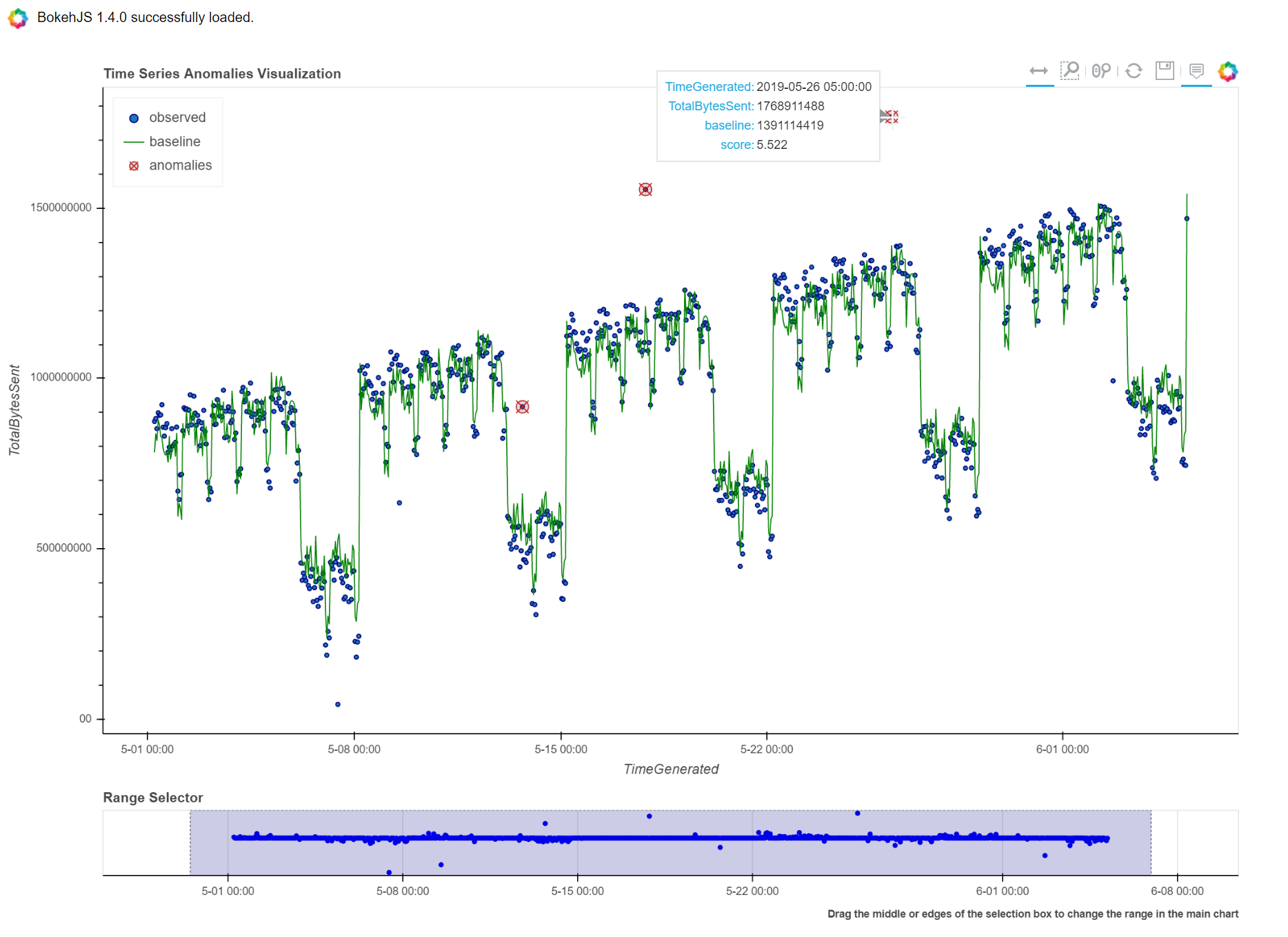
Time Series Anomalies Visualization
Time series anomalies once discovered, you can visualize with line chart
type to display outliers. Below we will see 2 types to visualize using msticpy function
display_timeseries_anomalies() via Bokeh library as well as using
built-in KQL render.
display_timeseries_anomalies.
display_timeseries_anomalies(data=timeseriesdemo, y= 'TotalBytesSent')
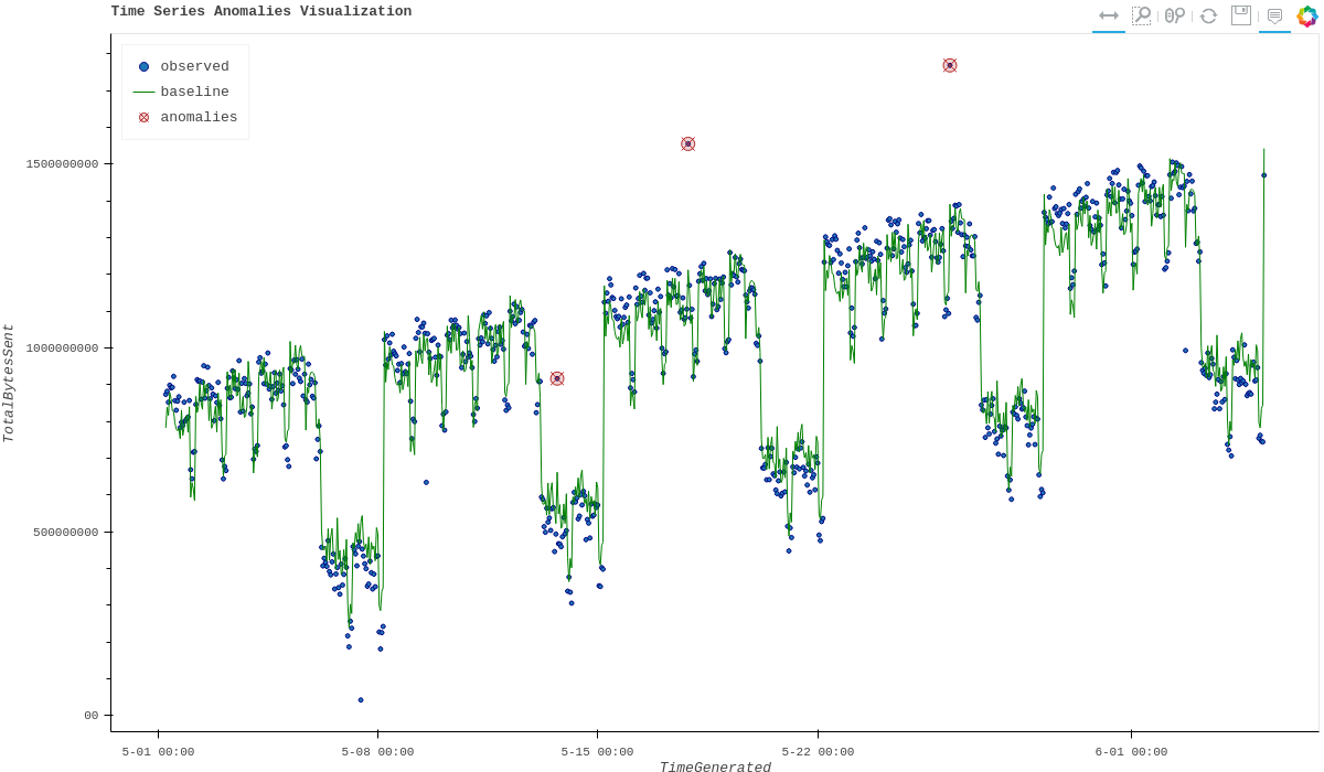
Exporting Plots as PNGs
To use bokeh.io image export functions you need selenium, phantomjs and pillow installed:
conda install -c bokeh selenium phantomjs pillow
or
pip install selenium pillow npm install -g phantomjs-prebuilt
For phantomjs see https://phantomjs.org/download.html.
Once the prerequisites are installed you can create a plot and save the
return value to a variable. Then export the plot using export_png
function.
from bokeh.io import export_png
from IPython.display import Image

# Create a plot
timeseries_anomaly_plot = display_timeseries_anomalies(data=timeseriesdemo, y= 'TotalBytesSent')

# Export
file_name = "plot.png"
export_png(timeseries_anomaly_plot, filename=file_name)

# Read it and show it
display(Markdown(f"## Here is our saved plot: {file_name}"))
Image(filename=file_name)
Here is our saved plot: plot.png
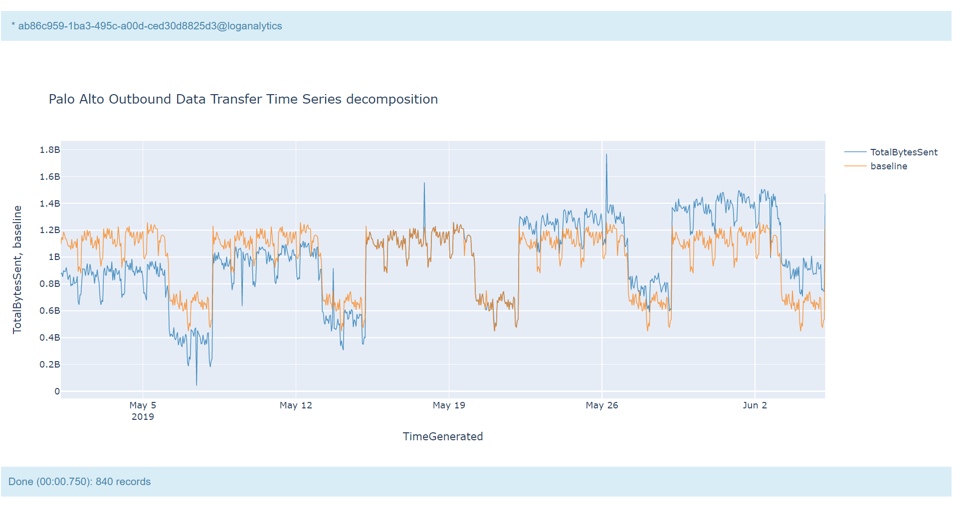
Using Built-in KQL render operator
Render operator instructs the user agent to render the results of the query in a particular way. In this case, we are using timechart which will display linegraph.
KQL Reference Documentation: - render
timechartquery = """
let TimeSeriesData = PaloAltoTimeSeriesDemo_CL
| extend TimeGenerated = todatetime(EventTime_s), TotalBytesSent = todouble(TotalBytesSent_s)
| summarize TimeGenerated=make_list(TimeGenerated, 10000),TotalBytesSent=make_list(TotalBytesSent, 10000) by deviceVendor_s
| project TimeGenerated, TotalBytesSent;
TimeSeriesData
| extend (baseline,seasonal,trend,residual) = series_decompose(TotalBytesSent)
| mv-expand TotalBytesSent to typeof(double), TimeGenerated to typeof(datetime),
  baseline to typeof(long), seasonal to typeof(long), trend to typeof(long), residual to typeof(long)
| project TimeGenerated, TotalBytesSent, baseline
| render timechart with (title="Palo Alto Outbound Data Transfer Time Series decomposition")
"""
%kql -query timechartquery